Week 4: 16/02/22

Table of Contents

Comments on Problem sheet A1

Question 2

I don’t have anything in particular to highlight for this question.

Question 3

• b) The key point here is that we are told the concentration is at a steady state so $dV/dt = f(V) = 0$. We know $\mu$ from the previous part of the question so we can sub in our values for $V,\mu$ into $$ \kappa=\mu V $$

• c) first solve for $I(t)$ then sub into $V(t)$ ode which can then be solved. Again, easiest in this case to use integrating factor. The written solutions go into a lot of detail by looking at $\mu>\delta$ and $\mu<\delta$ then $\mu\rightarrow\delta$ to show that $V$ is always positive. The key things to look at when we want to sketch the solution and then comment on it are:

  • Is $V$ always positive? (as the solutions show)
  • What does it look like near $t\approx0$? ($dV/dt>0$ so is increasing)
  • What does it look like as $t\rightarrow\infty$? ($V\rightarrow 0$)
  • Are there any turning points?

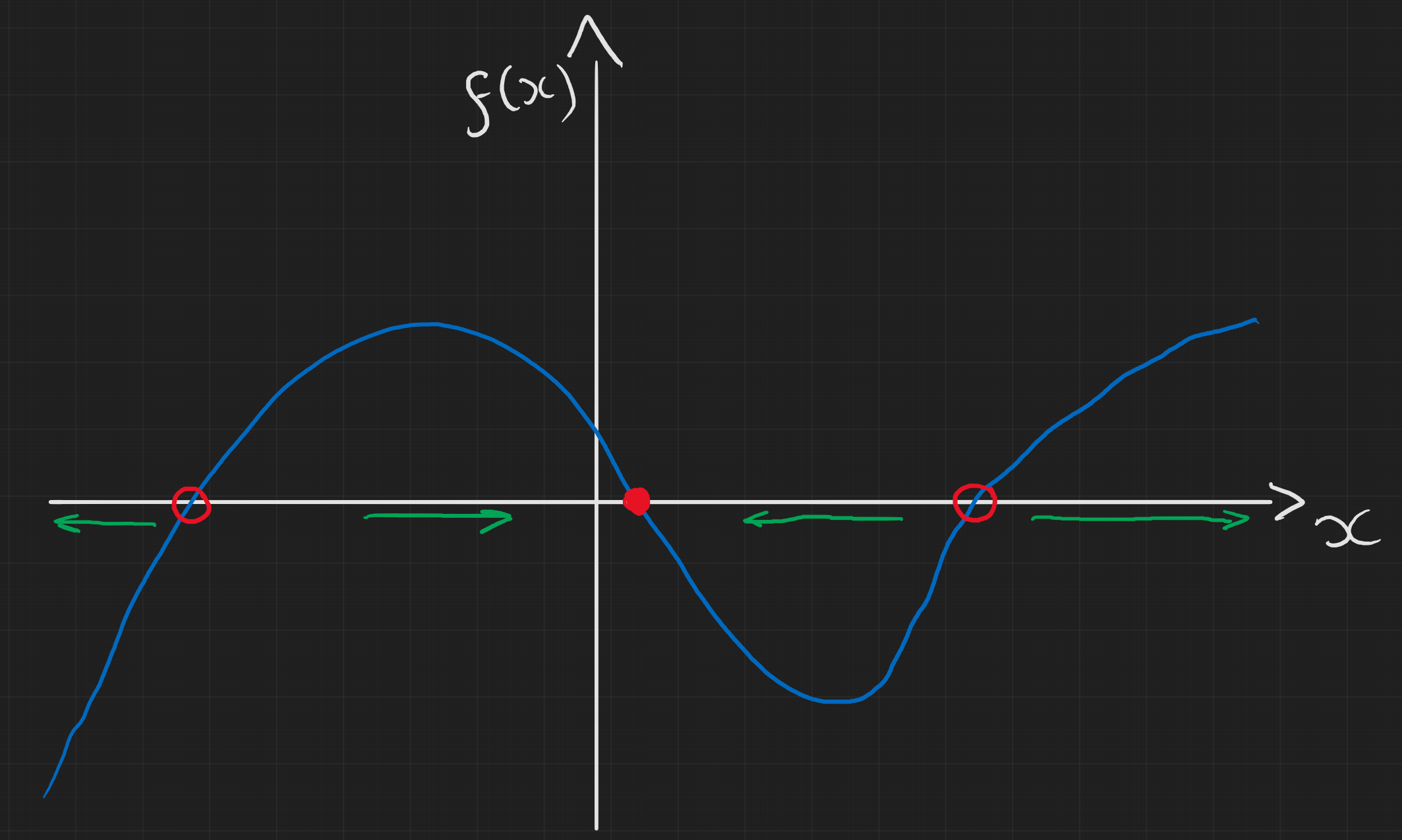
  We can infer that there is a turning point purely from the fact that $V$ starts off increasing from $0$ but will eventually return to $0$ so there must be a turning point which we can find explicity if needed. This gives us enough information to draw a sketch of the solution though which can be seen below for some arbitrary choice of $\delta,\mu$.

Outline of lecture content

Geometric Method

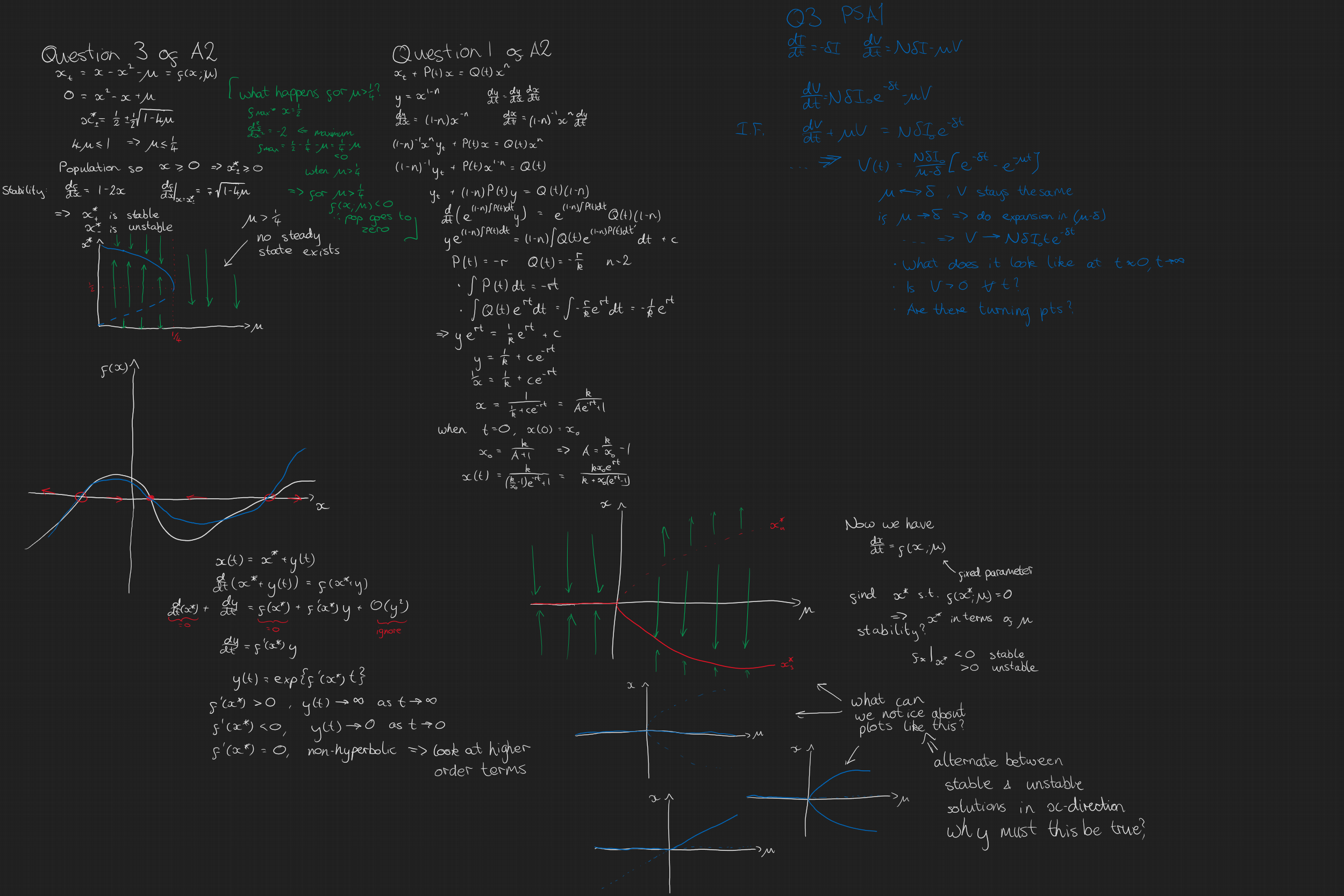
This picture should sum up the takeaways from this section in the notes. If $f(x)>0$ then $x$ by definition is increasing and so our system will move towards the right. Conversely if $f(x)<0$ then $x$ decreases and so we draw a left arrow instead. This then tells us the stability of our steady states located at $f(x)=0$. If the arrows point inwards then it’s stable and we can show this with a filled circle, if they point outwards then it’s unstable and we denote this with a hollow circle.

Linear Stability Analysis

There isn’t much to add here beyond what the lecture notes have.

Bifurcations

Now we have non-linear systems with some parameter $\mu$ and we want to know how the system behaves for different values of this parameter. We can still use the same techniques as before but now we get a rich understanding of a more general problem.

• Firstly, we can find the steady states, $x^*$, such that $f(x^*;\mu)=0$. This will give us some solutions for $x^*$ in terms of our parameter $\mu$.
• Next we need to make sure we know for what values of $\mu$, these solutions exist. When there is a range of values for which some solutions exist but do not outside this range, we get a bifurcation.
• We can then go ahead and plot these solutions in the allowed range in a plot of $x$ vs $\mu$.
• Finally, to determine the stability of these solutions, we use the linear stability method from before. If a solution is stable then $$ \frac{dx}{dt}|_{x^*}<0 $$ and the opposite is true for unstable solutions. If we have equality then the steady state is non-hyperbolic and we have to look at the higher derivaties.
• We then draw the unstable solutions with dashed lines and the stable ones with filled in lines

In the notes which are available at the top of this page, I’ve drawn a few examples of some bifurcations we might see. Some are a bit beyond what will be studied in the course but this gives an idea of the standard types of sketches we expect to see. Below is one such example.

Problem sheet A2

Question 1

This question does not really have anything conceptually new. The steps are just

• Use the substitution specified
• Use an integrating factor of $\exp(\int P(t) dt)$
• Obtain a solution for $y$ in terms of general $P(t),Q(t)$.
• Substitute in $P(t)=-r$, $Q(t)=-r/k$ and $n=2$.
• The rest is rearranging for $x(t)$ and putting in an initial condition of $x(0)=x_0$. Full working can be found in the solutions on moodle.

Question 3

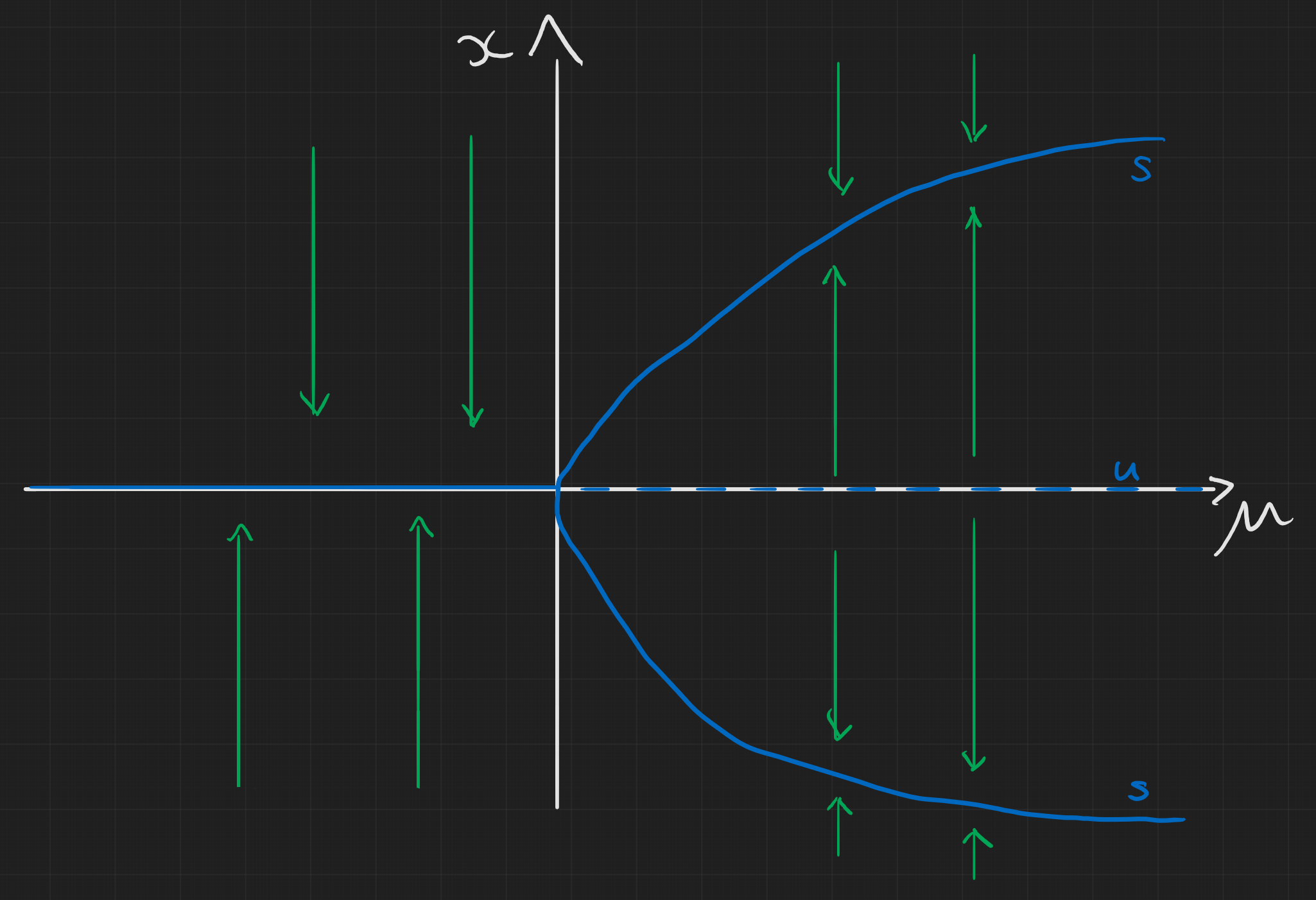
Following the steps I outlined before we first find that $$ x_{\pm}^* = \frac{1}{2}\left(1\pm\sqrt{1-4\mu}\right) $$ Remember we need to check the range in which these solutions are valid. $$\Rightarrow 4\mu\leq 1 \quad \Rightarrow \mu\leq\frac{1}{4}$$ Also we’re working with a population and a harvesting rate so $x>0,\mu>0$.

Next we find the stability of these steady states: $$ \frac{df}{dx} = 1 - 2x, \quad \Rightarrow \frac{dx}{dt}|_ {x^*{\pm}} = \mp\sqrt{1-4\mu} $$ so $x{+}^*$ is stable and $x_{-}^*$ is unstable.

We can also check what happens when $\mu\geq1/4$. There is a turning point at $x=1/2$, and we know it’s maximum since $$ \frac{d^2f}{dx^2} = -2 $$ Now, $$f\left(\frac{1}{2}\right)= \frac{1}{2}-\frac{1}{4}-\mu=\frac{1}{4}-\mu<0$$. Therefore $f(x;\mu)<0$ for $\mu>1/4$ and thus the population goes to $0$.

Below I’ve put a heatmap of $f(x;\mu)$, the boundary where it switches from light red to light blue gives us the steady state solutions and we can determine the stability too. Red means $f(x;\mu)<0$ so it’s like an arrow pointing down while blue is like an arrow pointing up.